SSD Object Detection with Focal Loss and Non Max Suppression.

We look at how Object Detection works with SSD and how we extend the YOLO model to perform better with a convolutional layer at the end.

Goal

The goal is to have a fast and reasonably accurate one-stage detector. Better accuracy is generally obtained with 2 stage detectors like R-CNN. The accuracy is upto 10-40% better. For single shot detectors like SSD and YOLO, we benefit from the speed and simplicity.

SSD Object Detection

The fundamental difference between the YOLO model described here and the model we explore today is that the last layer that we customise, is a bunch of convolutional layers.

Our loss function differs a little but it is infact a variation of the Binary Cross Entropy Loss function we used before.

The architecture

Our resnet layer returns returns an output of shape (512 x 7 x 7 ) this remains unchanged as long as we continue to use resnet34 as our base.

Our model now has some variations.

We create a simple convolutional layer as a starting point to use in our model.

class StdConv(nn.Module):
    def __init__(self, nin, nout, kernel_size=3, stride=2, padding=1, drop=0.5):
        super().__init__()
        self.conv = nn.Conv2d(nin, nout, kernel_size=kernel_size, stride=stride, padding=padding)
        self.bn = nn.BatchNorm2d(nout)
        self.drop = nn.Dropout(drop)
        
    def forward(self, x): return self.drop(self.bn(F.relu(self.conv(x))))

Our layer is a convutional layer which has

1. a Conv2d layer with a (3x3) kernel and a default stride of 2
2. We have a Dropoff of 0.5. The drop off values plays a big role in how well our model fits and I’ve tried this with values ranging from 0.5 to 0.58 with varying degrees of success. I suggest trying what values work best for you. I noticed training with higher dropouts allowed me to get around overfitting early when training the last layers.
3. We have a BatchNorm2d layer and a dropout. Our forward method does nothing special but note that it includes a ReLU after the convolution.

Similarly, we create an OutConv layer which represents the output. Our output now expects a set of coordinates representing the bounding box and the classification scores for each of our 21 classes (20 + background).

class OutConv(nn.Module):
    def __init__(self, k, nin, num_classes, bias):
        super().__init__()
        self.k = k
        self.oconv1 = nn.Conv2d(in_channels=nin, out_channels=((num_classes) * k), kernel_size=3, padding=1, bias=True)
        self.oconv2 = nn.Conv2d(nin, 4*k, 3, padding=1, bias=True)        
        
        
    def forward(self, x, debug=False):        
        _classes = self.oconv1(x)
        _coords = self.oconv2(x)
        if debug: print(f'[OutConv]: classes: {_classes.shape}, coords: {_coords.shape}')
                  
        classes = flatten_conv(_classes, self.k)
        coords = flatten_conv(_coords, self.k)
        if debug: print(f'[OutConv] Flattened classes: {classes.shape} Flattened coords: {coords.shape}')
            
        return [classes, coords]

We create 2 Conv2d layers which return the num_classes sized activations and 4*k sized activations. Assuming k=1 this would make sense as we have a 4 coordinates to represent the bounding box and num_classes probabilities representing each class within a bounding box in an image.

Our forward calls something called flatten_conv which simply reshapes the output

def flatten_conv(x, k, debug=False): 
    if debug: print(f'[Flatten] Input shape {x.shape}, k={k}')        
        
    bs, num_features, row, cols = x.shape
    flattened = x.view(bs, num_features//k, -1)
    
    if debug: print(f'[Flatten-2] Flattened shape {flattened.shape}')
        
    return flattened.permute(0,2,1)

The flatten_conv method simply returns tensors after reshaping them with the permute call. This gives us a two tensors of shape 128 x 189 x 4 for coordinates and 128 x 189 x 21 for classes.

1. The 128 represents our batch size
2. The final axis which are 4 and 21 represent the coordinates and the classification probabilities.
3. The 189 is something we arrive at because of the architecture we chose and the anchor box resolutions we adopted.

Batch Size

One of the things that I’ve often ignored as a meaningful hyper parameter is the batch size. Here is an interesting post by Kevin Shen on how batch size and learning rates affect the training cycle. I noticed that a bs of 128 was the one that worked best for me.

Anchor Boxes

Much like before our anchor boxes are the baseline template we create upfront to detect the image category of the entity that falls within those coordinates.

We use a fairly elaborate set of bounding boxes generated by this method

def get_scaled_anchors():    
    anc_grids = [4, 2, 1]
    anc_zooms = [0.7, 1., 1.3]
    anc_ratios = [(1., 1.), (1., 0.5), (0.5, 1.)]

    anchor_scales = [(anz*i,anz*j) for anz in anc_zooms 
                                        for (i,j) in anc_ratios]
    # *** Number of Anchor Scales
    k = len(anchor_scales)
    # ***************************

    anc_offsets = [2/(o*2) for o in anc_grids] #2 is the h,w in fastai 1.0 (-1,1)
    anc_x = np.concatenate([np.repeat(np.linspace(ao-1, 1-ao, ag), ag)
                            for ao,ag in zip(anc_offsets,anc_grids)])
    anc_y = np.concatenate([np.tile(np.linspace(ao-1, 1-ao, ag), ag)
                            for ao,ag in zip(anc_offsets,anc_grids)])
    anc_ctrs = np.repeat(np.stack([anc_x,anc_y], axis=1), k, axis=0)
    anc_sizes = np.concatenate([np.array([[2*o/ag,2*p/ag] 
                  for i in range(ag*ag) for o,p in anchor_scales])
                     for ag in anc_grids]) #2/grid * scale,2 is the h,w in fastai 1.0
    grid_sizes = tensor(np.concatenate([np.array([ 1/ag 
                  for i in range(ag*ag) for o,p in anchor_scales])
                      for ag in anc_grids])).unsqueeze(1) *2 #again fastai 1.0 h,w is 2
    anchors = tensor(np.concatenate([anc_ctrs, anc_sizes], axis=1)).float()

    print(f'K is {k}')
    return anchors, grid_sizes

Unlike our attempt at YOLO our anchor boxes have 3 different aspect ratios and grid sizes.

We end up with a total of 189 bounding boxes as a result. That’s where we get the 189 from.

A peak into the anchor boxes

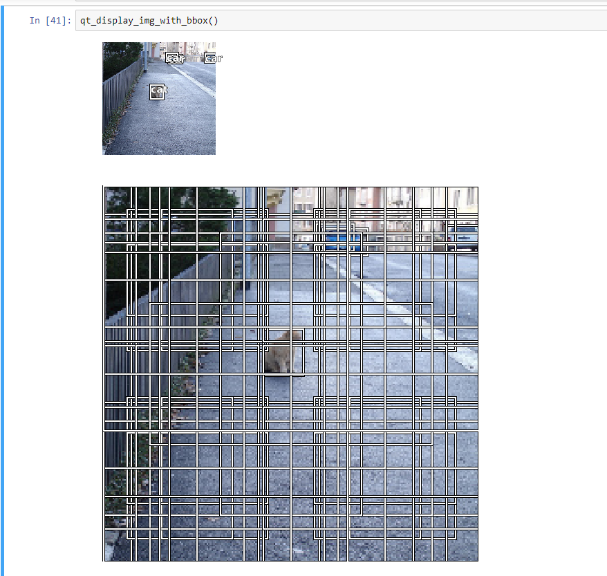
This gives us an idea of how the bounding boxes are organised for an image.

Shaping the model to yield 189 activations

The essence of model creation is to ensure the number of activations passed to the model’s loss function are of identical shape to be able to perform meaningful reductions. In our case our loss function has 2 components

1. Comparing the predictions of classes (using Binary Cross Entropy and Focal Loss)
2. Comparing the bounding box sizes with L1 loss.

For comparing the classes we need to ensure our tensors are shaped as 128x189x4 and 128x189x21

Our model looks like this.

class SSDHead(nn.Module):
    def __init__(self, k, bias, num_of_classes):
        super().__init__()
        self.drop = nn.Dropout(0.5)
        #self.sconv_1 = StdConv(2048, 1024, stride=1) #1024x7x7 (additinal)
        #self.sconv_2 = StdConv(1024, 512, stride=1) #512x7x7  (additinal)
        self.sconv0 = StdConv(512, 256, stride=1) #256x7x7
#       self.sconv1 = StdConv(256, 256, stride=1) #256x7x7 (additinal)
        self.sconv2 = StdConv(256, 256) #256x4x4
        self.sconv3 = StdConv(256, 256) #256x2x2
        self.sconv4 = StdConv(256, 256) #256x1x1
        self.out = OutConv(k, 256, num_of_classes, bias)
        
    def forward(self, x, debug=False):
        if debug: print(f'[SSDhead] input shape {x.shape}')
        x = self.drop(F.relu(x))
        if debug: print(f'[SSDHead-1] relu-dropout output shape {x.shape}')
        #x = self.sconv_2(self.sconv_1(x))    
        x = self.sconv0(x)
        if debug: print(f'[SSDHead-2] sconv0 output shape {x.shape}')
#         x = self.sconv1(x)
        x = self.sconv2(x)
        c1, bb1 = self.out(x)        
        if debug: 
            print(f'[SSDHead-3] sconv2 output shape {x.shape}')
            
        
        x = self.sconv3(x)
        c2, bb2 = self.out(x)
        if debug: 
            print(f'[SSDHead-4] sconv3 output shape {x.shape}')
            print(f'[SSDHead-4] c2 {c2.shape}  bb1: {bb2.shape}')
        
        x = self.sconv4(x)
        c3, bb3 = self.out(x)
        
        if debug: 
            print(f'[SSDHead-5] sconv4 output shape {x.shape}')        
            
            print(f'[SSDHead-5] c1 {c1.shape}  bb1: {bb1.shape}')
            print(f'[SSDHead-5] c2 {c2.shape}  bb1: {bb2.shape}')
            print(f'[SSDHead-5] c3 {c3.shape}  bb1: {bb3.shape}')
        
        c, bb = torch.cat([c1, c2, c3], dim=1), torch.cat([bb1, bb2, bb3], dim=1)        
        if debug: print(f'[SSDHead-6] concatenated shape c: {c.shape}, b:{bb.shape}')
            
        return [c, bb]
    

Let’s step through this one layer at a time

1. Our first input is the output of the resent34 layer which is of the shape 512x7x7
2. We run this through a ReLU and Dropout layer. This results in no change in shape.
3. We then pass the results x through our sconv0 layer. The sconv0 layer is StdConv(512, 256, stride=1) where it accepts 512 input features and returns 256 outputs with a stride one. Thus our output is now shaped as 256x7x7. Only a stride 2 halves the shape of the output activations.
4. It then passes through another StdConv layer sconv2 with a default stride of 2 this time resulting in a shape of 256x4x4. Since the input and out features remain the same.
5. We then pass this to the outlayer and store the values in c and bb variables.
6. So at each step the output of the coordinates is k* size_of_image. Since the size of the image is 4x4 after sconv2, 9x16 gives us 144 activations.
7. The one after sconv3 is 2x2 which after the out layer returns 36 activations.
8. And finally, sconv4 returns an image of 1x1 which returns 9. We concatentate all of them to get 189 activations for.
9. This, in essence is the crux to model building. If we now decide to go with resnet50 we simply uncomment the lines on top and run through OutConv the last few layers.

For resnet50

        #self.sconv_1 = StdConv(2048, 1024, stride=1) #1024x7x7 (additinal)
        #self.sconv_2 = StdConv(1024, 512, stride=1) #512x7x7  (additinal)

Loss function

Our loss function remains more or less the same apart from the addition of Focal Loss

def one_hot_embedding(labels, num_classes, debug=False):
    if debug: 
        print(f'labels: {labels} {labels.shape}')
        print(f'num_classes: {num_classes}')
        print(f'lables.data {labels.data}')
    return torch.eye(num_classes)[labels.data.cpu()]

class BCE_Loss(nn.Module):
    def __init__(self, num_classes):
        super().__init__()
        self.num_classes = num_classes

    def forward(self, pred, targ):
        """
        The t[:, 1:] and p[:, 1:] ensures the first class `background` is ignored in both target and predicted classes
        """        
        t = one_hot_embedding(targ, self.num_classes)[:, 1:]
        t= t.cuda()
        x = pred[:,1:]       
        w = self.get_weight(x,t,focal_loss=True) # for focal loss
        return F.binary_cross_entropy_with_logits(x, t, w, reduction='sum')/(self.num_classes - 1)
    
    def get_weight(self,x,t, focal_loss=False): 
        if not focal_loss: return None
        x,t = x.cpu(),t.cpu()
        alpha,gamma = 0.25,1.
        p = x.sigmoid()
        pt = p*t + (1-p)*(1-t)
        w = alpha*t + (1-alpha)*(1-t)
        return (w * (1-pt).pow(gamma)).cuda().detach()
    

Focal Loss

Most of my understanding of comes from this brilliant talk on Focal Loss Detection by Tsung-Yi Lin which goes on to describe Feature Pyramid network. I’ve summarized the talk in the next few paragraphs.

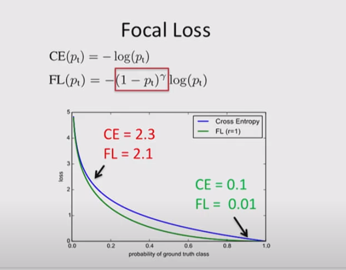
In object detection loss functions our goal remains to penalise incorrectly classified objects. But in most scenarios the breakdown of easy and hard examples is heavily imbalanced. The loss generated by a hard example may be significantly higher than that of an easy example. Thus the total loss of easy examples outweighs the total loss of the hard examples. However, the feedback from the hard examples are far more valuable in training the model.

Focal Loss is a modulated function which reduces the loss for easy examples more than for hard examples.

Our get_weights function contains two components alpha and gamma. gamma determines how much our loss function is going to focus on hard examples. So when gamma is 0 it behaves as before (negative log loss as in image).

The alpha parameter allocates different parameters to elements in the foreground and the background.

The values for alpha and gamma are from the paper which offers the values that work best. I’ve tried gamma from 1 to 2 and found the best results while using 1

Useful hints along the way while training

1. I’ve seen different notebooks approaching this differently but I didn’t bother normalising the target coordinates fit a 1x1 image. So no dividing by 224.
2. I trained for several epochs close to 35 * 7 epochs while i’ve seen some achieve decent results in much less.
3. Finding the best learning rates is something that still appears to be a ninja level skill to me but some priceless feedback from @Joseadolfo on the fastai forums helped me determine the best learning rates.
4. I approached it by periodically testing the classification and regression results after every 10 epochs but I expect there to be more sophisticated ways to approach it.

Non Max Suppression

This and this video seemed to be one of the better explanations I’ve found for non max suppression.

The objective of having NMS is to ensure we only show the best bounding boxes and classifications for an candidate based on the confidence. We select a threshold for how much confidence we need to present our result.

By candidate we refer to the top 100 (this could be any value) of the best overlaps as returned by our predictions.

Here we select the threshold before we pass it to nms

def process_nmf(idx, debug=True):
    '''
    Connects to the nmf algorith to filter out dupplicate bounding boxes
    ''' 
    # Minimun threshold for eliminating background noise
    min_thresh = 0.11   #0.25
    
    # Maximun threshold for eliminating duplicate boxes
    max_thresh = 0.32 
    
     # Extract predicted classes
    clas_pr, clas_ids = b_clas[idx].max(dim=1)

    
    # Mask Index of classes whose contents are over the noise level: 0 if the index contains no boxes, 1 if it does
    clas_pr = clas_pr.sigmoid()    
    
    # Calculate confidence score for Class Activations
    conf_scores = b_clas[idx].sigmoid().t().data      
    
    
    
    # Converts activation vectors to boxes. Shape: 189 x 4
    p_final_bbox = actn_to_bb(b_bb[idx].cpu(), anchors, grid_sizes=grid_sizes) 
    
    # lists for accumulating selected boxes and classes
    tot_bx, tot_cls = [], []
    
    scrd_cls_lst = data.classes.copy()
  
    # Loop across all classes
    for cl in range(0, len(conf_scores)):
        
        # Filter out Backgrounds and empty box arrays        
        c_mask = conf_scores[cl] > min_thresh         
        if c_mask.sum() == 0 or cl == 0: continue
        
        
        # scores for the selected class 
        scores = conf_scores[cl][c_mask] # Tensor 
           
        # These are active boxes. Ready to be processed by nmf
        boxes = p_final_bbox.cpu().index_select(dim=0,index=c_mask.nonzero().squeeze())
        
        # Run NMF
        ids, count = nms(boxes.data, scores, overlap=0.5, top_k=20)
        ids = ids[:count]
        
    
        
        # Filter all boxes & classes over the threshold and accumulate them in lists
        for i, (sc, bx) in enumerate(zip(scores, boxes.data[ids] )): 
                 
            tot_bx.append(bx)
            tot_cls.append(cl)
            # Create a scored label
            f = f'{i}: '           
            l = f'{data.classes[cl]} '
            s = '{0:.2f}'.format(sc) 
            sl = f+l+s
            # print('scored label: {} '.format(sl))
            scrd_cls_lst[cl] = sl

                
    if not tot_cls:
        print('Inferred Class list is empty. Image may be too faint.')
        return None, None, None  
    
    return torch.cat(tot_bx).view(-1, 4), torch.tensor((np.array(tot_cls))), scrd_cls_lst

I work with a low threshold of 0.11 which may not be what you need but it will try to identify as much as possible in the image. We also pass the amount of overlap (IoU) we expect which in our case is 0.5. I’ve used @Joseadolfo’s version of nmf here and updated the thresholds to suit my requirements.

The code

The final example lives here and I’ve retained all the different attempts and failures in this repository