Object Detection Basics

The fundamentals of understanding object detection with YOLO and SSD architectures.

Object detection revolves around a few main architectures such as YOLO (we’re referring to the older versions and not v3), SSD (Single Shot Detection) and FPN (Feature Pyramid Net). While this post focuses mainly on my understanding of YOLO and SSD here is a piece by Nick Zeng which beautifully explains how FPN works. Nick’s twitter is available here

Starting with Single Object detection.

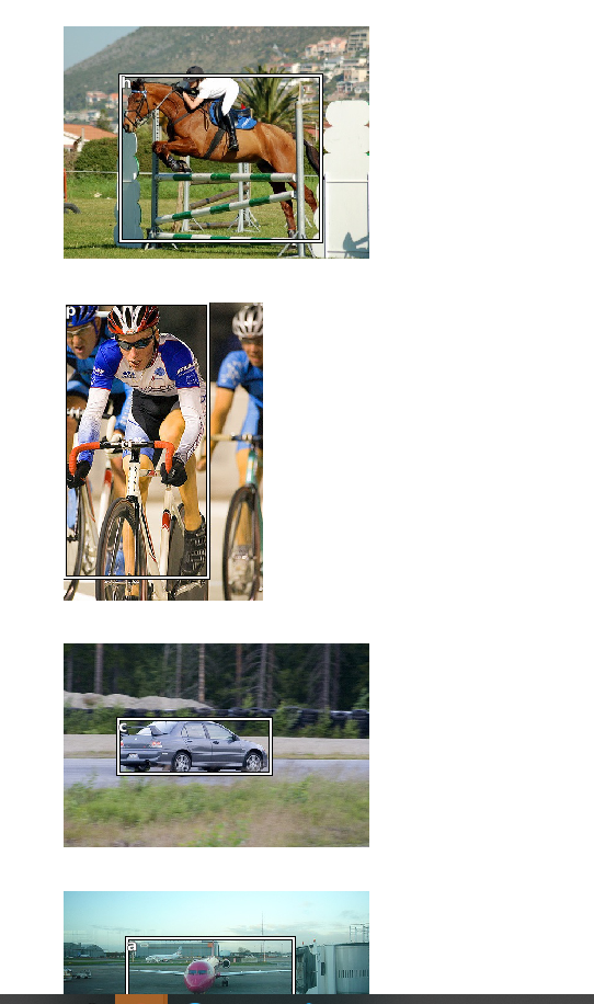
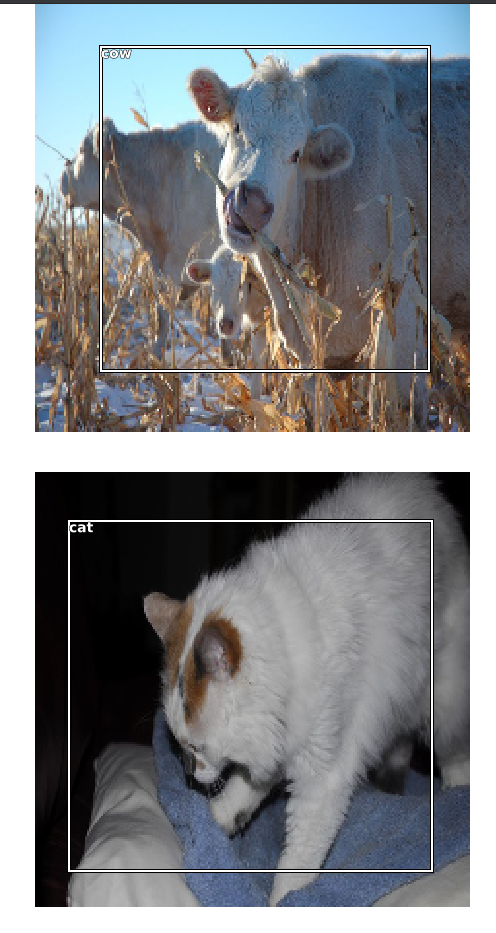
Here we focus mainly on detecting the largest object in each image. For example from our Pascal 2007 dataset here are few examples

The architecture

The core architecture remains very similar to the one used for transfer learning with MultiClass classification with resnet with one small change. Here our training dataset contains annotations containing the bounding boxes for the largest image with their associated category.

So our model needs to return two things

1. The category of the classified image
2. The bounding box of the image.

The classification part of the problem remains the same where we use Categorical Cross Entropy as our loss function. But the bounding box part of our output is a regression problem.

So after Resnet determines the classes of the largest image we need to run regression on our final layers and return both the class and the coordinates the identify the image.

So our new final layer would look like this

head_reg4 = nn.Sequential(
    Flatten(), 
    nn.ReLU(),
    nn.Dropout(0.5),    
    nn.Linear(25088, 256),
    nn.ReLU(),
    nn.BatchNorm1d(256),
    nn.Dropout(0.5),
    nn.Linear(256, 4+data.c)
)

This flattens the output received from the last resnet layer that would’ve been 512x7x7 (25088) so we end up with a flattened activation which we run through ReLU, Dropout, Linear a couple of times and output a tensor of shape (4+data.c)

Here 4 represents the 4 point coordinate which represents the top x,y and bottom x,y coordinates for our image. The data.c represents the number of categories in our dataset which in the case of Pascal dataset is 20 + 1 (The +1 represents background)

So with that out of the way our model needs to be able to evaluate the loss of the regression and the classification in a meaningful way.

Loss function

So our loss function can be split into 2 parts again. One for classification for which we’ll use the Categorical Cross Entropy loss and L1Loss for the regression part of the problem.

:
def detn_loss(input, target, targ_cls):    
    bbox_targ = target
    bbox_inp, cat_inp = input[:, :4], input[:, 4:]    
    bbox_inp = bbox_inp[:, None]    
#   print(f' bbox_inp {bbox_inp}, bbox_targ {bbox_targ}')
    bbox_inp = torch.sigmoid(bbox_inp) * 224
    bbox_targ = torch.sigmoid(bbox_targ) * 224
#   print(f' bbox_inp2 {bbox_inp}, bbox_targ2 {bbox_targ}')
    return F.l1_loss(bbox_inp, bbox_targ) + F.cross_entropy(cat_inp, targ_cls.flatten())* 20


def detn_l1(input, target, _targ_cls):    
    bbox_targ = target
    bbox_inp = input[:, :4]
    bbox_inp = bbox_inp[:, None]
    bbox_inp = torch.sigmoid(bbox_inp) * 224
    bbox_targ = torch.sigmoid(bbox_targ) * 224
    return F.l1_loss(bbox_inp, bbox_targ).data

The inputs to our loss function is always in the form prediction, target. Since we’re using Fastai’s handy ObjectItemList our target values are already returned as target coordinates and classes seperately.

data = ObjectItemList.from_folder(JPEGS_PATH)
data = data.split_by_files(list(vimages))
data = data.label_from_func(get_y_func_largest, label_cls=StubbedObjectCategoryList) 
data = data.transform(get_transforms(max_zoom=1, max_warp=0.05, max_rotate=0.05, max_lighting=0.2), 
                      tfm_y=True, size=224, resize_method=ResizeMethod.SQUISH)
data = data.databunch(bs=16, collate_fn=bb_pad_collate)
data = data.normalize(imagenet_stats)

However, we need to ensure we separate the coordinates and the classes for our prediction because our model returns just one vector for the form (4+data.c)

Now, it’s passed into L1Loss and CrossEntropy and we multiply with 20 to ensure the scales are equivalent.

Train and predict

Here’s the notebook with the training and predictions.

MultiObject detection with a simple 4x4 grid of anchor boxes.

For single object detection we use a linear layer which returns a vector of the shape (4+data.c). This is the characteristic difference between YOLO and SSD. SSD uses a convolutional layer which is carefully designed to return an output layer that maps to the number of anchor boxes we choose. We’ll get into the details of what we mean by anchor boxes but the essential difference is that YOLO uses a linear output layer returning a vector while SSD uses a convolutional layer at the end to return the information of the classification and bounding boxes.

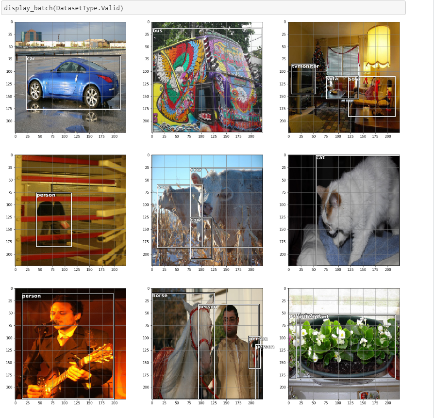
Our goal with this exercise is to be able to detect every object within the 21 categories for an image

Anchor boxes

Let’s split our image into a $4x4$ grid which generates 16 sections for an image. Each section may contain a category of the object. So our anchor boxes are bounding boxes for 224x224 image spread evenly.

Each image can be viewed as being made up 16 evenly spaced grids which may hold a category of image. The coordinates of the grid are the coordinates of the anchor box. Think of this as the template for our multi object classification problem. Our goal now is to classify the images that fall into each grid.

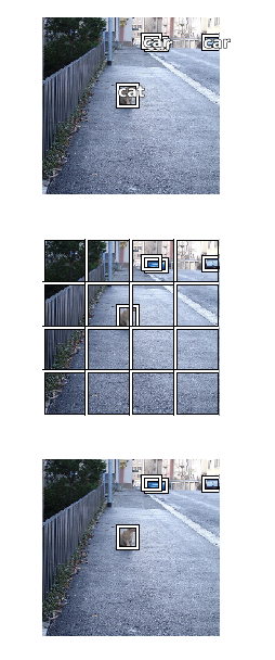
This image shows the presence of a cat and cars. The following snippet creates the 4x4 grid we need.

from torch.autograd import Variable as V

anc_grid = 4
k = 1


anc_offset = 1/(anc_grid*2) # 0.125
four_point_grid = np.linspace(anc_offset, 1-anc_offset, anc_grid)
anc_x = np.repeat(four_point_grid, anc_grid)
anc_y = np.tile(four_point_grid, anc_grid); anc_y

# anchor centers
anc_centers = np.stack([anc_x, anc_y], axis=1);
anc_ctrs = np.tile(anc_centers, (k, 1))

# anchor sizes
anc_sizes = np.array([[1/anc_grid,1/anc_grid] for i in range(anc_grid*anc_grid)])

#anchor coords and height and width
anchors = np.concatenate([anc_ctrs, anc_sizes], axis=1); anchors
anchors = torch.Tensor(anchors)
anchors = V(anchors, requires_grad=False).float()

# grids
grid_sizes = torch.Tensor(np.array([1/anc_grid])); grid_sizes
grid_sizes = V(grid_sizes, requires_grad=False).unsqueeze(1)

The architecture

The architecture for our SSD model now contains a convolutional layer that we attach at the end of the resent model.

class OutConv(nn.Module):
    def __init__(self, k, nin, num_classes, bias):
        super().__init__()
        self.k = k
        self.oconv1 = nn.Conv2d(in_channels=nin, out_channels=((num_classes) * k), kernel_size=3, padding=1)
        self.oconv2 = nn.Conv2d(nin, 4*k, 3, padding=1)
        self.oconv1.bias.data.zero_().add_(bias)
        
    def forward(self, x):        
        return [flatten_conv(self.oconv1(x), self.k), 
                flatten_conv(self.oconv2(x), self.k)]


class SSDHead(nn.Module):
    def __init__(self, k, bias, num_of_classes):
        super().__init__()
        self.drop = nn.Dropout(0.25)
        self.sconv0 = StdConv(512, 256, stride=1) 
        self.sconv2 = StdConv(256, 256)
        self.out = OutConv(k, 256, num_of_classes, bias)
        
    def forward(self, x, debug=False):
        if debug: print(f'[SSDhead] input shape {x.shape}')
        x = self.drop(F.relu(x))
        if debug: print(f'[SSDHead-1] relu-dropout output shape {x.shape}')
        x = self.sconv0(x)
        if debug: print(f'[SSDHead-2] sconv0 output shape {x.shape}')
        x = self.sconv2(x)
        if debug: print(f'[SSDHead-3] sconv2 output shape {x.shape}')
        x = self.out(x)
        if debug: print(f'[SSDHead-4] out output shape {np.array(x).shape}')
        return x                

So our model contains 2 StdConv layers following a Dropout. The StdCov layers is a standard convolutional layer made up of conv2d, BatchNorm2d and a Dropout

class StdConv(nn.Module):
    def __init__(self, nin, nout, kernel_size=3, stride=2, padding=1, drop=0.1):
        super().__init__()
        self.conv = nn.Conv2d(nin, nout, kernel_size=kernel_size, stride=stride, padding=padding)
        self.bn = nn.BatchNorm2d(nout)
        self.drop = nn.Dropout(drop)
        
    def forward(self, x): return self.drop(self.bn(F.relu(self.conv(x))))

The most interesting aspect of the SSDHead is the OutConv which accepts an input of shape 256, 4, 4 from the sconv2 and returns a list of 2 elements.

The list is essentially the results we need. It consists of 2 parts

self.oconv1 = nn.Conv2d(in_channels=nin, out_channels=((num_classes) * k), kernel_size=3, padding=1)

1. The convolution which returns the clasification result, where it takes the 256x4x4 input and returns one of the 21 classes. (It actually returns a score for each of the 21 classes)

 self.oconv2 = nn.Conv2d(nin, 4*k, 3, padding=1)

1. And another conv2d which accepts the same input and returns 4 coordinates. So our output again is returning a list of coordinates and classes. However, for each image we’re now return 16 such coordinates and classes. One for each grid cell from our anchor box template.

How did we arrive at 16 coordinates

Let’s follow this with an example

[SSDhead] input shape torch.Size([16, 512, 7, 7])
[SSDHead-1] relu-dropout output shape torch.Size([16, 512, 7, 7])
[SSDHead-2] sconv0 output shape torch.Size([16, 256, 7, 7])
[SSDHead-3] sconv2 output shape torch.Size([16, 256, 4, 4])
[SSDHead-4] out output shape (2,)

1. Our resnet layer outputs a shape of (512 x 7 x 7 ). This forms the input to our SSDHead
2. SSDHead has a ReLU followed by a Dropout which doesn’t change the shape of our activations so we remain at (512 x 7 x 7)
3. We have a StdConv which accepts a 512 input features and returns 256. But it’s a stride 1 conf so our we’re still at (7x7) for our image dimensions.
4. We have another StdConv which accepts the 256 and returns 256 features but this is a stride 2 conv and hence we have (4x4) activation. Now if this is flattened it would give us 16 activations which is what OutConv does. Thus returning a list of length 2.
5. The values with our list are of shape
   1. 16x(c) - 16 x 16 x 21 (which is our classes)
   2. 16x(4) - 16 x 16 x 4 (and our coordinates)

The loss function

The loss function is the tricky bit and took me over 2 weeks to fully understand how each component worked. For simplicity we’ll avoid additional concepts like Focal Loss and NMS in this post.

Let’s analyze the entire set of functions in the context of the inputs

ef get_nonzero(bbox,classes):
    """
    Accepts a target_coords and classes
    1. bbox: target_coords 
    2. classes: target_classes
    
    It ensures thes shape is [whatever size x 4], ie: groups of 4 coords
    It checks if the difference between x2 - x1 is > 0  and filters all the `nonzero` values indexes
    
    And using those indexes `bb_keep` returns those from the orignal `bbox` and `classes` arrays
    """
    bbox = bbox.view(-1,4)/224
    retain_idxs = ((bbox[:,2]-bbox[:,0])>0).nonzero()[:,0]
    return bbox[retain_idxs],classes[retain_idxs]

# Getting rid of -ve values 
def normalize(bbox, debug=False):
    if debug:
        print(f'[NORMALIZE] bbox: {bbox} bbox.sum: {bbox.sum()} bbox.std: {bbox.std()} bbox.mean: {bbox.mean()}')
    return (bbox+1./2.)


def hw2corners(ctr, hw): 
    """
    Given the center and the height and width returns the 4 corners of a bounding box
    """
    return torch.cat([ctr-hw/2, ctr+hw/2], dim=1)

def intersect(box_a, box_b):
    """
    for a given set of pred_coords and anchor boxes
    1. `max_xy` finds the innermost top left coordinates. That is min(x) and min(y)
    2. `min_xy` finds the furthest bottom right,  `bottom left`. That is max(x) and max(y)
    3. `clamp` ensures the values are greater than 0
    4. `inter * inter` computes the areas of the two sets of coordinates and returns the overlapping area.
    """
    top_left = torch.min(box_a[:, None, 2:], box_b[None, :, 2:])
    bottom_right = torch.max(box_a[:, None, :2], box_b[None, :, :2])
    inter = torch.clamp((bottom_right - top_left), min=0)
    return inter[:, :, 0] * inter[:, :, 1]

def box_area(b): 
    return ((b[:, 2]-b[:, 0]) * (b[:, 3]-b[:, 1]))

def jaccard(box_a, box_b, debug=False):
    """
    Intersection over union
    """
    if debug:
        print(f'[JACCARD] box_a: {box_a}')
        print(f'[JACCARD] box_b: {box_b}')
    inter = intersect(box_a, box_b)
    union = box_area(box_a).unsqueeze(1) + box_area(box_b).unsqueeze(0) - inter
    return inter / union


def actn_to_bb(actn, anchors, grid_sizes):
    """
    Given a set of 
    1. actn: activations from a prediction
    2. anchors: Anchors computed beforehand for a default image of size 1x1. (anchors)
    3. grid_sizes: Grid size for each of the bounding box on the default image
    4. The tanh converts the values between -1 and 1
    Anchors return the list of (anchor_centers, anchor_sizes)
    
    """
    actn_bbs = torch.tanh(actn)
    actn_centers = (actn_bbs[:,:2]/2 * grid_sizes) + anchors[:,:2]
    actn_hw = (actn_bbs[:,2:]/2+1) * anchors[:,2:]
    return hw2corners(actn_centers, actn_hw)

def map_to_ground_truth(overlaps, debug=False):
    """
    `overlaps.max(1)`:
        1. returns the overlap of the activations with the ground truth anchor boxes
        2. Which is returns the largest overlaps (area) and anchor box index       
    
    `overlaps.max(0)`:
        1. returns overlap of activations overlap with respect to each of the
           ground truth boxes
        2. For every anchor box in our anchors the overlap area and the activation that overlapped
     
     The function assigns every anchor box to a ground truth label.
    """
    if debug: print(f'[MAP_TO_GROUND_TRUTH] overlaps: {overlaps}')
    overlap_val, overlap_idx = overlaps.max(1)    
    gt_overlap, gt_idx = overlaps.max(0) 
    
    if debug: 
        print(f'[MAP_TO_GROUND_TRUTH] overlap_val:{overlap_val}, overlap_idx:{overlap_idx}')
        print(f'[MAP_TO_GROUND_TRUTH] gt_overlaps: {gt_overlap}, gt_idx:{gt_idx}')
        
    gt_overlap[overlap_idx] = 1.99
    for ix, overlap_index in enumerate(overlap_idx):
        gt_idx[overlap_index]=ix
        
    if debug:
        print(f'[MAP_TO_GROUND_TRUTH] gt_overlaps: {gt_overlap}')
        print(f'[MAP_TO_GROUND_TRUTH] gt_idx: {gt_idx}')      
            
    return gt_overlap, gt_idx   
    
    

def ssd_1_loss(p_cls, p_coords, t_cls, t_coords, debug=False):
    t_coords, t_cls = get_nonzero(t_coords, t_cls)    
    t_coords = normalize(t_coords)   
    actn_centers_hw = actn_to_bb(p_coords, anchors.cuda(), grid_sizes.cuda())  
    if debug:        
        print(f'[SSD_1_LOSS] t_coords = {t_coords}')
        print(f'[SSD_1_LOSS] p_coords = {p_coords}')
        print(f'[SSD_1_LOSS] actn_centers_hw = {actn_centers_hw}')
    anchor_centers = anchors[:, :2]
    anchor_hw = anchors[:, 2:]
    anchor_corners = hw2corners(anchor_centers.cuda(), anchor_hw.cuda())  
    overlaps = jaccard(t_coords, anchor_corners.cuda())
    try:
        gt_overlap, gt_idx = map_to_ground_truth(overlaps)
    except Exception as e:
        return 0., 0.
    
    gt_classes = t_cls[gt_idx]
    positive_overlaps = gt_overlap > 0.4
    positive_overlaps_idx = torch.nonzero(positive_overlaps)[:, 0]
    gt_bbox = t_coords[gt_idx]
    loc_loss = (
        actn_centers_hw[positive_overlaps_idx] - gt_bbox[positive_overlaps_idx]
    ).abs().mean()
    class_loss_func = BCE_Loss(data.c)
    class_loss = class_loss_func(p_cls, gt_classes)
    return loc_loss, class_loss  
    

def ssd_loss(pred, targ, target_class, debug=False):    
    pred_classes, pred_coords = pred       
    
    # For each set of 16x4 coords and 16x(num_classes) per image in a batch compute the loss
    regression_loss, class_loss = 0., 0.
    for p_cls, p_coords, t_coords, t_cls in zip(pred_classes, pred_coords, targ, target_class):        
        l1_loss, cls_loss = ssd_1_loss(p_cls, p_coords, t_cls, t_coords)
        regression_loss += l1_loss
        class_loss += cls_loss 
    
    if debug:        
        print(f'regression_loss: {regression_loss}, class_loss: {class_loss}')
     
    return regression_loss + cls_loss

So we know that our loss function receives the predictions and target as input. We also know from the Single Object Detection part that Fastai’s ObjectItemList class splits the target coordinates and target classes for us.

The entry point of our loss is the ssd_loss method. Which receives a single batch of images. Assuming our batch size is 16 our inputs for a batch would be of the shape

1. 16 x 16 x 21 classes
2. 16 x 16 x 4 coordinates.

So now we need to determine the loss but since we usually compute loss in batches (our batch size is 16) our existing setup won’t work. Our situation is slightly different given we have 16 tiny grids each containing an image and a set of coordinates. Our loss is the loss of each of these grids put together.

So, we need to allow our ssd_loss to be able to compute the loss for each anchor box grid in the template.

1. For the target value coordinates (not our predictions), we determine the overlaps using the jaccard index. The overlap is the interesection of the image coordinates in the original image (ground truth) with respect to the anchor box grids in our template. We’re trying to determine which anchor boxes overlap with the ground truth images.
2. The jaccard method returns scores of the overlap and the box it overlaps with.
3. If a positive prediction has greater than 0.4 (40%) overlap then we get the corresponding label (class of the box). So now we know what the class is for each box. So now we can safely assume that a grid in the anchor box template would represent a specific category.
4. We now get the predicted activations in terms of the anchors box coordinates using the actn_to_bb function. This returns the predicted activations as bounding box coordinates. What that means is for each prediction we have the activations that are now returned as bounding box coordinates mapping to the 4x4 anchor box template. We now compare the grids that mapped positively with a category by running them through our loss function.
5. Now our bounding box loss function is just the L1Loss which is the distance between the coordinates.

loc_loss = (
        actn_centers_hw[positive_overlaps_idx] - gt_bbox[positive_overlaps_idx]
    ).abs().mean()

1. For our classification we rely on Binary Cross entropy with logits which is just BCE with a sigmoid activation upfront. (Here is a neat cheatsheet to understand Cross Entropy losses from Sebastian Raschka’s blog)
2. Finally we simply add the values for each grid and repeat across batches.

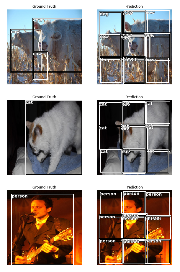
However, our outputs aren’t the best. This is largely because of the anchor grids we chose. In the subsequent posts, I’ll venture into grids with different zooms, a modified model architecture and better predictions.

The code

1. Single Object detection - YOLO
2. [Multi Object Detection - SSD