Cheatsheet
This post is some of the details I use as a quick reference when things slip my mind. It’s a snapshot of frequently used operations, jargon and methods that trip me while working with data, Pytorch or Fastai. A lot of writing here contains typos and the intent was to have a quick reference to the concept.
Valuable Links
- Count and sort with Pandas https://stackoverflow.com/questions/40454030/count-and-sort-with-pandas
- Using
isinfor selecting from a list https://stackoverflow.com/questions/40454030/count-and-sort-with-pandas
Topics
- Collaborative filtering with Fastai https://towardsdatascience.com/collaborative-filtering-with-fastai-3dbdd4ef4f00
Valuable snippets
Dropping duplicates
dedup_df = without_reviews_df.drop_duplicates(subset=['product_id', 'user_nickname', 'review_text'], keep='first',
                inplace=False)
dedup_df
Group by
grouped_by_category_df = dedup_df.groupby(by='product_category_primary')
grouped_by_category_df
Group by user_nickname in sorted order and count the number of products in each group and return nlargest groups
x = (relevant_makeup_df.groupby(by=['user_nickname'], sort=True)['product']
                       .count()
                       .nlargest(38679))
Find percentage of missing values in the dataset
relevant_makeup_df.isna().sum()Finds the all thenanornullvalues in the dataset for each column and sums it uprelevant_makeup_df.shape[0]Fetches the number of rows in the dataset and divides the result of 1 and multiples by 100 to make it percentage
relevant_makeup_df.isna().sum()/relevant_makeup_df.shape[0] * 100
Find and assign all not null values to a dataframe for a specific column
# For each group - in this case for user `Mochapj`
d = grouped_by_user_df.get_group('Mochapj')

# Find all the `skinConcerns` that are not null
skin_concerns_df = d[d['skinConcerns'].notnull()]

# Fetch the unique value if only one
skin_concerns_df['skinConcerns'].unique()[0]

# select all records from `relevant_make_df` for the user `Mochapj` and assign the attribute `skinConcerns` with the value `aging`
relevant_makeup_df.loc[relevant_makeup_df['user_nickname']=='Mochapj', 'skinConcerns'] = 'aging'

# List and view the updated values
relevant_makeup_df.loc[relevant_makeup_df['user_nickname']=='Mochapj']
Drop na values for a specific column in a dataframe
df.dropna(subset=['EPS'], how='all', inplace=True)
What is an Embedding
An embedding matrix is a weight matrix that is randomly generated by the Pytorch’s nn.Embedding module which creates a bunch of random values
So an embedding is just a matrix that you can lookup to obtain the weight.
In collaborative filtering there is an additional bias added to the weights.
class EmbeddingDotBias(Module):
    "Base dot model for collaborative filtering."
    def __init__(self, n_factors:int, n_users:int, n_items:int, y_range:Tuple[float,float]=None):
        self.y_range = y_range
        (self.u_weight, self.i_weight, self.u_bias, self.i_bias) = [embedding(*o) for o in [
            (n_users, n_factors), (n_items, n_factors), (n_users,1), (n_items,1)
        ]]

    def forward(self, users:LongTensor, items:LongTensor) -> Tensor:
        dot = self.u_weight(users)* self.i_weight(items)
        res = dot.sum(1) + self.u_bias(users).squeeze() + self.i_bias(items).squeeze()
        if self.y_range is None: return res
        return torch.sigmoid(res) * (self.y_range[1]-self.y_range[0]) + self.y_range[0]
If you notice the forward block the weights for the users is multiplied with the weight for the items and a random bias is added to the user and weights.
The torch.sigmoid is the non-linearity added to ensure the result stays between the output values. Think between 0 and 5 for a movie rating system
What is weight decay
Weight decay penalises complexity by subtracting the square of the weights of the parameters and multiples it with a constant
This is so that the best loss is not substituting the values of the parameters with 0
Hence wd is usually e-1 or e-01
Standard SGD
Here the following things happen
y = ax + b
Where m is the slope and b is the intercept
- Loss is calculated by the
msefunction which subtracts the(y' - y) ** 2and finds themeanof it - We assume the value of
def mse(y_hat, y):
    return ((y_hat-y)**2).mean()

a = nn.Parameter(a); a

def update():
    y_hat = x@a
    loss = mse(y, y_hat)
    if t % 10 == 0: print(loss)
    loss.backward()
    with torch.no_grad():
        a.sub_(lr * a.grad)
        a.grad.zero_()
Here the gradient is the rate of change of loss with respect to the change in weights.
Here $a$ represents the weights in each layer.
\(a_t = a_{t-1} - (lr * \frac{dLoss}{da})\)
SGD with weight decay
def update(x,y,lr):
    wd = 1e-5
    y_hat = model(x)
    # weight decay
    w2 = 0.
    for p in model.parameters(): w2 += (p**2).sum()
    # add to regular loss
    loss = loss_func(y_hat, y) + w2*wd
    loss.backward()
    with torch.no_grad():
        for p in model.parameters():
            p.sub_(lr * p.grad)
            p.grad.zero_()
    return loss.item()
What is momentum
Momentum is a constant that is used to multiply the derivative which a.gradient or p.gradient
in the earlier example in way where it adds momentum to the direction in which the model is learning
assuming b = 0.9 (beta/momentum)
- So assuming for epoch 1 the gradient was 0.59 and epoch 2 the gradient was 0.74 the calculation for the new weight for a b would multiply the 0.59 (previous epoch) with 0.9 thus retaining the old momentum and multiply gradient of epoch 2 with 0.1 and subtract the weights
Thus maintaining directional momentum. (momentum = 0.9 is the standard)
Loss functions
- SGD which uses Mean squared error
- Adam
- RMSProp
RMSProp
RMSPRop is very similar to Adagrad, with the aim of resolving Adagrad’s primary limitation. Adagrad will continually shrink the learning rate for a given parameter (effectively stopping training on that parameter eventually). RMSProp however is able to shrink or increase the learning rate.
RMSProp will divide the overall learning rate by the square root of the sum of squares of the previous update gradients for a given parameter (as is done in Adagrad). The difference is that RMSProp doesn’t weight all of the previous update gradients equally, it uses an exponentially weighted moving average of the previous update gradients. This means that older values contribute less than newer values. This allows it to jump around the optimum without getting further and further away.
Further, it allows us to account for changes in the hypersurface as we travel down the gradient, and adjust learning rate accordingly. If our parameter is stuck in a shallow plain, we’d expect it’s recent gradients to be small, and therefore RMSProp increases our learning rate to push through it. Likewise, when we quickly descend a steep valley, RMSProp lowers the learning rate to avoid popping out of the minima.
Adam
Adam (Adaptive Moment Estimation) combines the benefits of momentum with the benefits of RMSProp. Momentum is looking at the moving average of the gradient, and continues to adjust a parameter in that direction. RMSProp looks at the weighted moving average of the square of the gradients; this is essentially the recent variance in the parameter, and RMSProp shrinks the learning rate proportionally. Adam does both of these things - it multiplies the learning rate by the momentum, but also divides by a factor related to the variance.
Universal Approximation Theorem
When a combination of matrix (Weights) multiplications are stacked together with activation functions it can solve any arbitarily complex function to a high level of accuracy.
The loss function is what the back propagation relies on where it goes back to adjust the weights. The adjustment is essentially the gradient subtracted from the weights.
What are dropoffs
Use regularisation rather than reducing than parameters. We periodically drop off activations randomly based on a parameter. emb_drop and p. emb_drop drops off certain embeddings while p drops activations.
last_learner = tabular_learner(data, layers=[1000,500], ps=[0.001,0.01], emb_drop=0.04,
                        y_range=y_range, metrics=accuracy)
p in tabular_learner
It’s form of regularisation. p in tabular_learners is the probability of dropping
activations for each layer. It’s specified on a per layer basis. p=[0.001, 0.01]
The common value is 0.5. The layer activations are dropped off with the probability of p
Dropouts aren’t used at the time of testing. Only during training. The library handles it.
layers in tabular_learner
It’s the number of attributes you want to assign for each feature (input parameter). It defines the shape of the parameter matrix that the input will be multiplied with
You can specify multiple layers for tabular data. layers=[100, 50]
emb_drop in tabular_learner
Embedding dropoffs deletes the outputs of the activations of certain embeddings at random with some probability
Predictions for tabular learner
for index, row in test_df.iloc[0:50].iterrows():
    actual = row['rating']
    prediction = last_learner.predict(row)
    prediction_ratios = prediction[2].numpy()
    scores = [(c, k) for c, k in zip(last_learner.data.train_dl.classes, prediction_ratios)]
    top_scores = sorted(scores, key=lambda x: x[1], reverse=True)[:2]
    first_score = top_scores[0][1]
    second_score = top_scores[1][1]

    if first_score > 0.65:
        print(f'Sure - a: {actual} p: {prediction[0]} r: {prediction_ratios}')
    else:
        print(f'Unsure a: {actual} p*: {top_scores[0][0], top_scores[1][0]} r: {scores}')
What is BatchNormalisation
It reduces something called Internal Covariant Shift. Math has proved that it doesn’t reduce internal covariant shift and why it works is not because of internal covariant shift
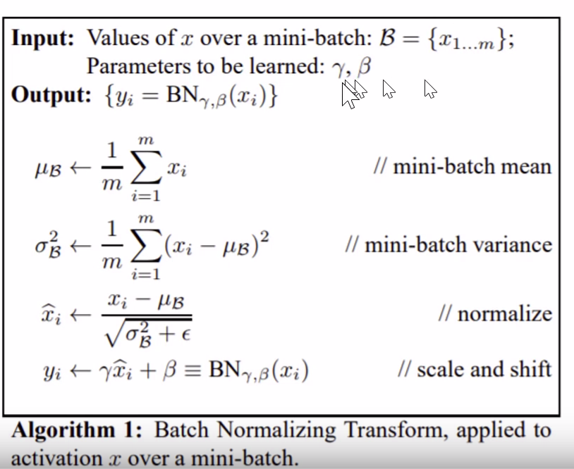
- For each mini batch
xwhich is activations, first we find the mean - Find the variance of all the activations
- We normalize the value that is
(values - mean / standard deviation) - Scale and shift where we add a bias term and another variable like a bias term which is multipled instead of adding. Hence
scaled - It’s a used in continuous parameters. It’s a form of regularization.
Convolution2D
Convolution2D essentially scans the pixels of an image as a 2x2 (as defined) matrix and multiples the values of each pixel with a weight and reduces a 2x2 matrix of pixels into a single value.
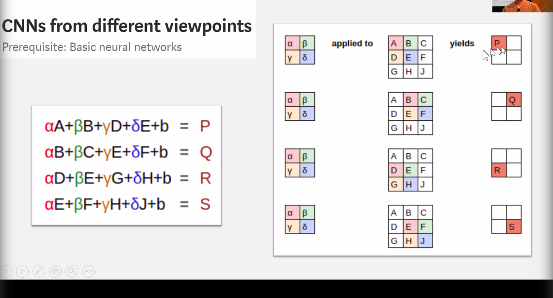
In the above image the weights for alpha, beta, gamma and theta represent the weights identifying certain colors and reducing the result to a 2x2 matrix
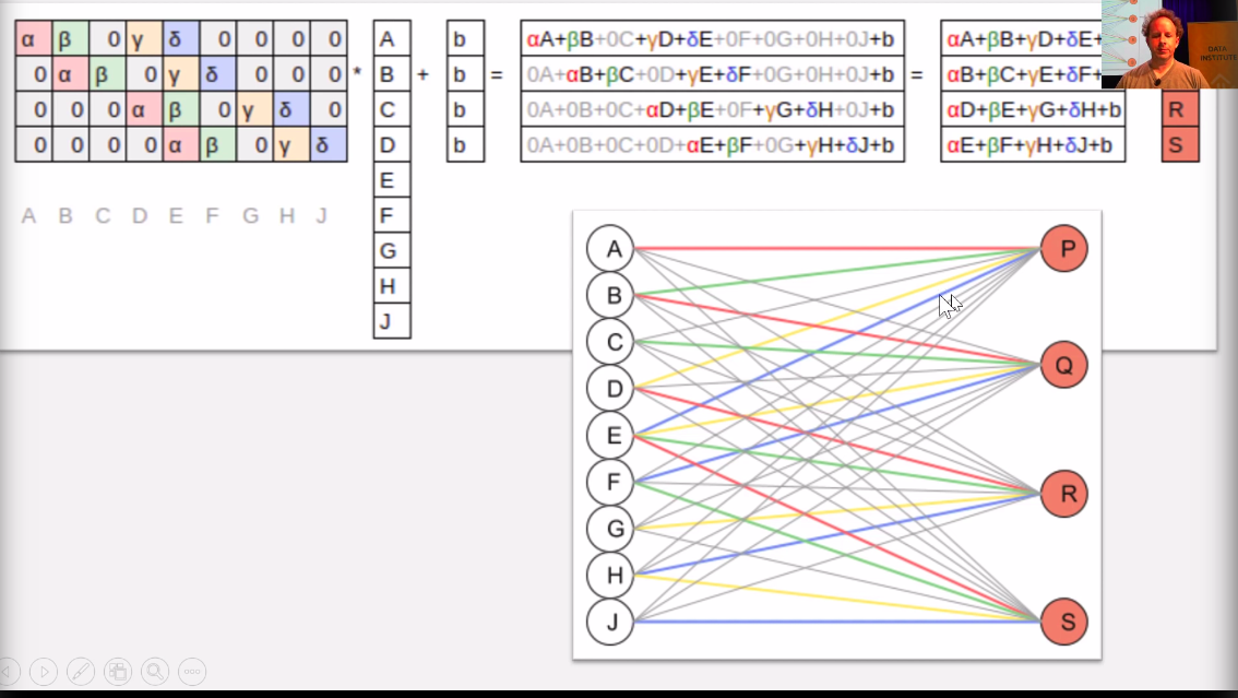
This image represents how the image matrix having
[
    [a, b, c],
    [d, e, f],
    [h, i, j]
]
is now flattened into a 1 dimensonal tensor [a, b, c, d, e, f, g, h, i, j]. THe weights are called the kernel
The b in the example represents the bias.
Learning Rates
When we pass
fit(1, 1e-3)
Every layer is trained with this learning rate
Discrimative learning rates
When we pass a slice with a single value the final layers get the value of 1e-3 but the all the layers before get 1e-3 divided by 3
fit(1, slice(1e-3))
When it’s
fit(1, slice(1e-5, 1e-3))
When 2 values are passed the first layers get (1e-5) and the subsequent layers get the layers get a gradually changing learning rate in the order of (1e-3)/2
Kaiming Initialisation
The process of initialising weights which yield a standard deviation of 1 and mean close to 0
Essentially it suggests that given
- A matrix of shape nxm (say 50,000 rows by 784 columns) like MNIST a good initialisation for weight matrices is
Assuming we want nh hidden layers or attributes (nh=50 for this example)
nh=50
w = torch.rand(m, nh)/math.sqrt(nh)
This would result in a weight matrix that provides us with a mean of 0 and a standard deviation of 1 when the activation for the network is a ReLu
import torch, math
torch.rand(784, 50)/math.sqrt(784)
tensor([[0.0292, 0.0176, 0.0236,  ..., 0.0146, 0.0024, 0.0097],
        [0.0249, 0.0037, 0.0325,  ..., 0.0228, 0.0183, 0.0339],
        [0.0320, 0.0271, 0.0021,  ..., 0.0319, 0.0205, 0.0293],
        ...,
        [0.0234, 0.0118, 0.0051,  ..., 0.0259, 0.0341, 0.0027],
        [0.0008, 0.0269, 0.0101,  ..., 0.0331, 0.0341, 0.0064],
        [0.0322, 0.0173, 0.0029,  ..., 0.0299, 0.0224, 0.0220]])
Broadcasting
How the underlying matmul within pyTorch works.
The thing about using broadcasting for multiplications is that it transposes each column of a and multiples it with the entire matrix b as columnar multiplication and sums it up to get the same result
So in the following example, consider matrices a and b
a = tensor([[1., 2.], [3., 5.], [4., 6.]])
b = tensor([[1., 3., 5., 7.], [2., 4., 6. ,8.]])
a.shape, b.shape
(torch.Size([3, 2]), torch.Size([2, 4]))
a[0, None].shape
torch.Size([1, 2])
The expected output for standard matrix multiplication is this
a.matmul(b)
tensor([[ 5., 11., 17., 23.],
        [13., 29., 45., 61.],
        [16., 36., 56., 76.]])
Our matrices is are shaped as
ar, ac = a.shape
br, bc = b.shape

a.shape, b.shape
(torch.Size([3, 2]), torch.Size([2, 4]))
The matmul method within pyTorch uses broadcasting to achieve higher computational speeds by passing the logic to the AL10 layers where it’s implemented in.
The method looks like this
def matmul(a,b):
    ar,ac = a.shape
    br,bc = b.shape
    assert ac==br
    c = torch.zeros(ar, bc)
    for i in range(ar):
#       c[i,j] = (a[i,:]          * b[:,j]).sum() # previous
        c[i]   = (a[i  ].unsqueeze(-1) * b).sum(dim=0)
    return c
Breaking down line number 13 which does the actual multiplication. He row 0 of matrix a is
a[0], a[0].shape
(tensor([1., 2.]), torch.Size([2]))
It does a a[0].unsqueeze(-1) to introduce a dimension and converts the row into a column.
What this means is the matrix is now shaped differently
a[0].unsqueeze(-1), a[0].unsqueeze(-1).shape
(tensor([[1.],
         [2.]]),
 torch.Size([2, 1]))
So now our matrix which was of shape (2,) is now of shape (2, 1).
Now the expected output of row[0] in matrix c is [ 5., 11., 17., 23.]
This is what a[i].unsqueeze(-1) * b does
a[0].unsqueeze(-1) * b
tensor([[ 1.,  3.,  5.,  7.],
        [ 4.,  8., 12., 16.]])
We now sum the two rows in the column dimension to get a single row of outputs
(a[0].unsqueeze(-1) * b).sum(dim=0)
tensor([ 5., 11., 17., 23.])
The loop essentially does this for each row of matrix a to generate rows of matrix c