Trying a different approach on this one by using Jupyter notebooks to generate a more visual document.

Quick Glace at the API
Terminology used across blogs and videos that can be confusing
SVD - Concepts and Examples
Other decomposition approaches

Quick Glance at how the API works

# Fastai imports to import pd, np, scipy etc.

from fastai import *
from fastai.core import Path

a1 = np.array([[1,2, 3], [1, 4, 1], [2, 3, 5]])
print(a1)
from scipy.linalg import svd
U, s, Vh = svd(a1, full_matrices=True)
U, Vh
(U * s) @ Vh

[[1 2 3]
 [1 4 1]
 [2 3 5]]

array([[1., 2., 3.],
       [1., 4., 1.],
       [2., 3., 5.]])

np.sum(U[:, 2]**2)

1.0000000000000007

Terminology

These are terms that are frequently used when discussing SVD.

Matrix Factorisation

Is a process of decomposing a matrix into two matrices that when run through a dot product result in the original matrix.

Orthogonal Matrix

An orthogonal matrix is one which when multipled with it’s transpose returns an Identity matrix

\[AA^t = A^tA = I\]

Diagonal Matrix

A diagonal matrix is one which has non-zero values in it’s diagonal

Column Orthonormal

The columns of the matrix are Eculidean length 1. Which means if you compute the sum of squared values of each column it’ll be 1.

a1 = np.array([[1,2, 3], [1, 4, 1], [2, 3, 5]])
print(a1)

[[1 2 3]
 [1 4 1]
 [2 3 5]]

from scipy.linalg import svd

U, s, Vh = svd(a1, full_matrices=True)

print(U)

array([[-0.466533,  0.184235, -0.865103],
       [-0.445706, -0.893781,  0.050018],
       [-0.763998,  0.408917,  0.499093]])

np.sum(U[:, 2]**2)
1.0000000000000007

Orthogonal

Any two columns of two matrices (say U and V), their dot product would be 0

Single Value Decomposition

What is SVD

The goal of SVD is to discover latent features present in a document. It’s the most widely used approach for recommendation systems.

It does not care about what the latent features are and does not expect the creator of the recommendor system to define the categories/concepts that define the product (or movies, music, books, etc). This system identifies these categories and assigns relevant weights depending upon the inputs provided by users. The inputs usually are ratings, likes, downvotes etc.

How does it work

The basis of the approach here is the understanding that each product is made up of N categories. To use the movie analogy here let’s say $Movie1$ is composed of $n$ categories at varying weights.

That is

\[Movie1 = (W_1 * Concept1) + (W_2 * Concept_2 ) + .... + (W_n * Concept_n)\]

where our concepts could be comedy, thriller, action, horror etc, meaning the movie is 70% comedy, 20% drama and 10% action.

Similary a user can be defined as someone who different categories/concepts to varying degress.

That is

\[User1 = (UW_1 * Concept1) + (UW_2 * Concept_2 ) + .... + (UW_n * Concept_n)\]

Visualising it as a problem

Let’s assume that the input information is provided to us as the following dataFrame

ratings = np.array([[3, 5, 4, 1, 1],
              [2, 2, 1, 4, 5],
              [3, 3, 5, 4, 3]])

movie_labels = ['Star Wars', 'Departed', 'Saving Pvt Ryan', 'Home Alone', 'Love Actually']
users = ['User1', 'User2', 'User3']
df = pd.DataFrame(ratings, columns=movie_labels, index=users)
df

	Star Wars	Departed	Saving Pvt Ryan	Home Alone	Love Actually
User1	3	5	4	1	1
User2	2	2	1	4	5
User3	3	3	5	4	3

So the SVD based factorisation returns 3 values $U$, $E$ and $V$

Where

$U$ is the left singular matrix
$E$ is the diagonal matrix (is a diagnonal matrix where the values of the diagonal are represented in decreasing order)
$V$ is the right singular vector

Our ratings matrix can therefore be represented as

\[ratings = (U * E) @ D\]

Computing the values of $U$, $E$ and $V$

from scipy.linalg import svd

U, E, V = svd(ratings, full_matrices=True)

pd.DataFrame(U, columns=['Concept1', 'Concept2', 'Concept3'], index=['User1', 'User2', 'User3'])

	Concept1	Concept2	Concept3
User1	-0.533328	0.673748	-0.511493
User2	-0.508224	-0.738581	-0.442952
User3	-0.676217	0.023714	0.736321

Our $E$ matrix can be viewed as representing the strength of each concept.

pd.DataFrame(E, index=['Concept1', 'Concept2', 'Concept3'])

	0
Concept1	12.012443
Concept2	4.690892
Concept3	1.922695

Our $V$ matrix can be viewed as representing the relationship between a movie and concept.

Since we have more movies the algorithm identifies additional concepts that those movies could be attributed to.

pd.DataFrame(V[:3], columns=movie_labels, index=['Concept1', 'Concept2', 'Concept3'])

	Star Wars	Departed	Saving Pvt Ryan	Home Alone	Love Actually
Concept1	-0.386689	-0.475485	-0.501365	-0.438803	-0.424818
Concept2	0.131153	0.418411	0.442342	-0.465950	-0.628455
Concept3	-0.109960	-0.642018	0.620318	0.344300	-0.269044

Shape of these matrices

So $rating$ is a $3x5$ matrix

$U$ is a $3x3$ matrix
$V$ is a $3x1$ matrix
$E$ is a $5x5$ matrix

Now we can visualise our $U$ matrix as a set of identified concepts to users.

Checking if U, V are orthonormal

Orthonormal is when the sum of the squares of the values of any column equal 1

np.sum(V[:][0] ** 2)

0.9999999999999999

np.sum(U[:][0] ** 2)

1.0000000000000002

Checking the decomposition of U and V is of the original input

The $E$ matrix is a diagonal matrix that is presently returned as a 3, 1 matrix. The problem for us now is that to reconstruct the original matrix we need to be able to multiply the matrices $U, E, V$

The shape of these however are in the for $U (3x3)$, $E (3,1)$ which if we convert to a diagnoal matrix would be $(3x3)$ and $V (5x5)$.

So we reshape our $E$ to be a $(3x5)$ to do this and call it $S$

Create an 0 value matrix of the shape $(3x5)$

   S = np.zeros((ratings.shape[0], ratings.shape[1]))
   S

 array([[0., 0., 0., 0., 0.],
     [0., 0., 0., 0., 0.],
     [0., 0., 0., 0., 0.]])

Feed the newly created diagonal matrix into $S$

 S[:ratings.shape[0], :ratings.shape[0]] = np.diag(E)
 S

 array([[12.012443,  0.      ,  0.      ,  0.      ,  0.      ],
       [ 0.      ,  4.690892,  0.      ,  0.      ,  0.      ],
       [ 0.      ,  0.      ,  1.922695,  0.      ,  0.      ]])

Our new shapes look like this

 U.shape, Sigma.shape, V.shape

 ((3, 3), (3, 5), (5, 5))

Now multiply to validate the factorization

 U @ S @ V

 array([[3., 5., 4., 1., 1.],
       [2., 2., 1., 4., 5.],
       [3., 3., 5., 4., 3.]])

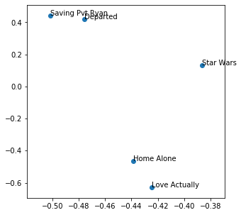
Visualising the movies as concepts

Based on the first 2 concepts our graph shows the Saving Pvt Ryan and Deoarted are similar, which would be a fair assement given they’re more action oriented while Star Wars has a more Scifi theme to it. Similarly Home Alone and Love Actually have a more family theme to them.

concept1 = V[:][0]
concept2 = V[:][1]


fig, ax = plt.subplots(figsize=(5, 5))
ax.scatter(concept1, concept2)

for idx, movie in enumerate(movie_labels):
    ax.annotate(movie, (concept1[idx], concept2[idx]))

png

Other matrix factorization methods that you may stumble upon.

While it’s not essential to know how this happens, it’s useful in visualising what is actually happening behind the scenes during the matrix factorisation process. A lot of times the terms such as orthonormal categories can trip one over while trying to follow tutorials that are more mathematical in nature.

Most of the actual computation is handled by scipy and sklearn so it’s safe to skip this section and look at the examples.

There are multiple ways in which matrices can be decomposed.

LU Decomposition

In this a matrix $A$ in decomposed into two matrices $L$ and $U$ where $L$ is considered to have the “Lower” trigular and U the upper triangular. The problem with LU decomposition is that it works on nxn matrices only. The outcome we end up with is $L @ U = A$ and $U @ L \neq A$

So for a matrix of the form
\[A = \begin{bmatrix} 1 & 5 & 12 \\ 1 & 2 & 3 \\ 2 & 4 & 3 \end{bmatrix}\]
Where $L$ and $U$ define our decompositions
\[L = \begin{bmatrix} 1 & 0 & 0 \\ L_{21} & 1 & 0 \\ L_{31} & L_{32} & 1 \end{bmatrix}\] \[U = \begin{bmatrix} U_{11} & U_{12} & U_{13} \\ 0 & U_{22} & U_{23} \\ 0 & 0 & U_{32} \end{bmatrix}\]
And finally,
\[\begin{bmatrix} 1 & 0 & 0 \\ L_{21} & 1 & 0 \\ L_{31} & L_{32} & 1 \end{bmatrix} X \begin{bmatrix} U_{11} & U_{12} & U_{13} \\ 0 & U_{22} & U_{23} \\ 0 & 0 & U_{32} \end{bmatrix} = \begin{bmatrix} 1 & 5 & 12 \\ 1 & 2 & 3 \\ 2 & 4 & 3 \end{bmatrix}\]
The transformations are achieved by using the row manipulation operations described here

LU example

from scipy.linalg import lu

A = np.array([[1, 5, 12], 
              [1, 2, 3], 
              [2, 4, 3]])
A

array([[ 1,  5, 12],
       [ 1,  2,  3],
       [ 2,  4,  3]])

Here P is the permutation matrix which represents the row swaps such that $PA=LU$

P, L, U = lu(A)
print(P)
print("")
print(L)
print("")
print(U)

P @L @ U == A

[[0. 1. 0.]
 [0. 0. 1.]
 [1. 0. 0.]]

[[1.  0.  0. ]
 [0.5 1.  0. ]
 [0.5 0.  1. ]]

[[ 2.   4.   3. ]
 [ 0.   3.  10.5]
 [ 0.   0.   1.5]]





array([[ True,  True,  True],
       [ True,  True,  True],
       [ True,  True,  True]])