Principal Component Analysis (PCA)

What is it?

It's a means of preserving information in reduced dimensions. 

What this effectively means is that in scenarios where we have a dataset with a large number of features (columns, usually), it gets harder to visualize the information and removing features may mean losing information.

In situations where the relationship between features is not obvious and we’re trying to reduce the number of features to have fewer relationships to deal with, PCA provides a means to extract features where a new variable is created which can be thought of as a combination of a set of features that are important (while discarding less important features.)

Why would we need it?

1. It makes it easy to visualize information on higher order features.
2. Possibly reduce noise
3. Make it easier to store and process easily. (Think space and time to compute)

What are Eigen Values and Eigen Vectors

While for most ML operations we won’t need one to understand what Eigen values and Eigen Vectors are directly, a quick run through of the broad concept could be handy. This youtube video by intrigano is in my opinion one of the best explanations that makes it easy to comprehend the PCA bits we’re about to deal with.

Essentially, the vectors that are characteristic to a transformation are referred to as Eigen Vectors.

What happens during PC computation

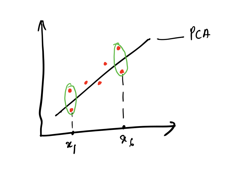
Consider the points in red as the values on a two dimensional plane, if we try to reduce the features by trying to map those points on either the X or Y axis we end up losing some data. Note the points in green are lost when plotted on the X-Axis. What computing Principal Component (incorrectly named as PCA in the diagram) does is it migrates the points towards the largest variance.

This in turn returns attributes that are a combination of multiple features.

Trying this with a real dataset.

Our problem dataset is the Tottenham Hotspurs squad dataset from 2018-2019 season of the English Premier league. Extracted from the footystats website. This dataset is freely available.

Since this dataset contains information about players from the entire league (i.e: every player who participated in the tournament from every team) we narrow it down to make it more relevant.

1. Get the dataset

   df = pd.read_csv(DATA_PATH/'players-2018-to-2019-stats.csv')
   df.head()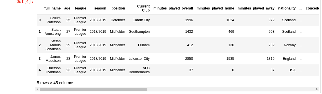
   

   

2. Extract Tottenham players

   tottenham_df = df[df['Current Club'] == 'Tottenham Hotspur']
   tottenham_df.head()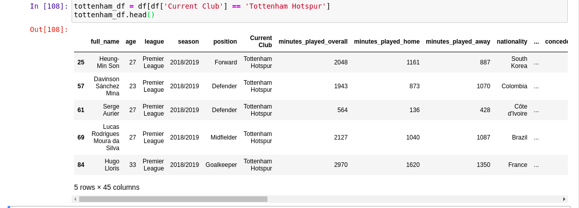
   

   

3. Change the index and drop league and club information since we’re working with only one league and club.

   tottenham_df.set_index('full_name')
   tottenham_df.drop(columns=['league', 'Current Club'], inplace=True)
   tottenham_df.head()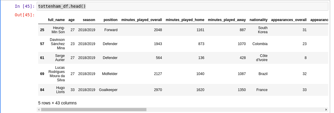
   

   

4. Encode categorical variables like nationality and Player position and get rid of the equivalent columns from the dataset

   from sklearn.preprocessing import LabelEncoder
   encoded_team_df = tottenham_df.copy()
   label_encoder = LabelEncoder()
   encoded_positions = label_encoder.fit_transform(tottenham_df['position'])
   encoded_nationality =  label_encoder.fit_transform(tottenham_df['nationality'])
   encoded_team_df['encoded_position'] = encoded_positions
   encoded_team_df['encoded_nationality'] = encoded_nationality
   encoded_team_df.drop(columns=['position', 'season', 'nationality'], inplace=True)
   

5. Scale values

   from sklearn.preprocessing import StandardScaler
   x_std = StandardScaler().fit_transform(encoded_team_df)
   pd.DataFrame(x_std)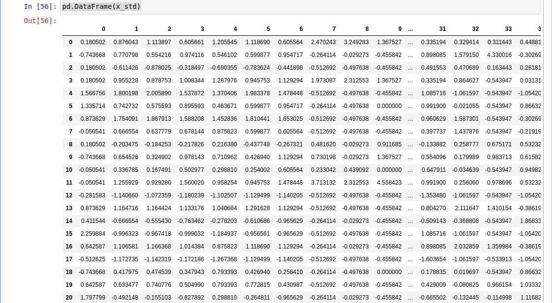
   

   

6. We could also manually compute the covariance matrix and the eigen values but this is not really needed as sklearn provides a built in function that computes PCA directly. It’s safe to skip 6 to 7

   features = x_std.T
   covariance_matrix = np.cov(features)
   

7. Now we find the eigen values and eigen vectors. This is what the line in the diagram represented.

   eig_vals, eig_vecs = np.linalg.eig(covariance_matrix)
   

8. We compute the principal components

   from sklearn import decomposition
   pca = decomposition.PCA(n_components=3)
   sklearn_pca_x = pca.fit_transform(x_std)
   pca_df = pd.DataFrame(sklearn_pca_x, columns=['pca1', 'pca2', 'pca3'])
   pca_df
   

Trying to interpret what attributes it could’ve clubbed together.

We plot the values of 2 PC on a chart and try to analyse what it could mean

fig, ax = plt.subplots(figsize=(20, 20))

ax.scatter(pca1, pca2)

for i, player_name in enumerate(encoded_team_df.index.tolist()):
    ax.annotate(player_name, (pca1[i], pca2[i]))

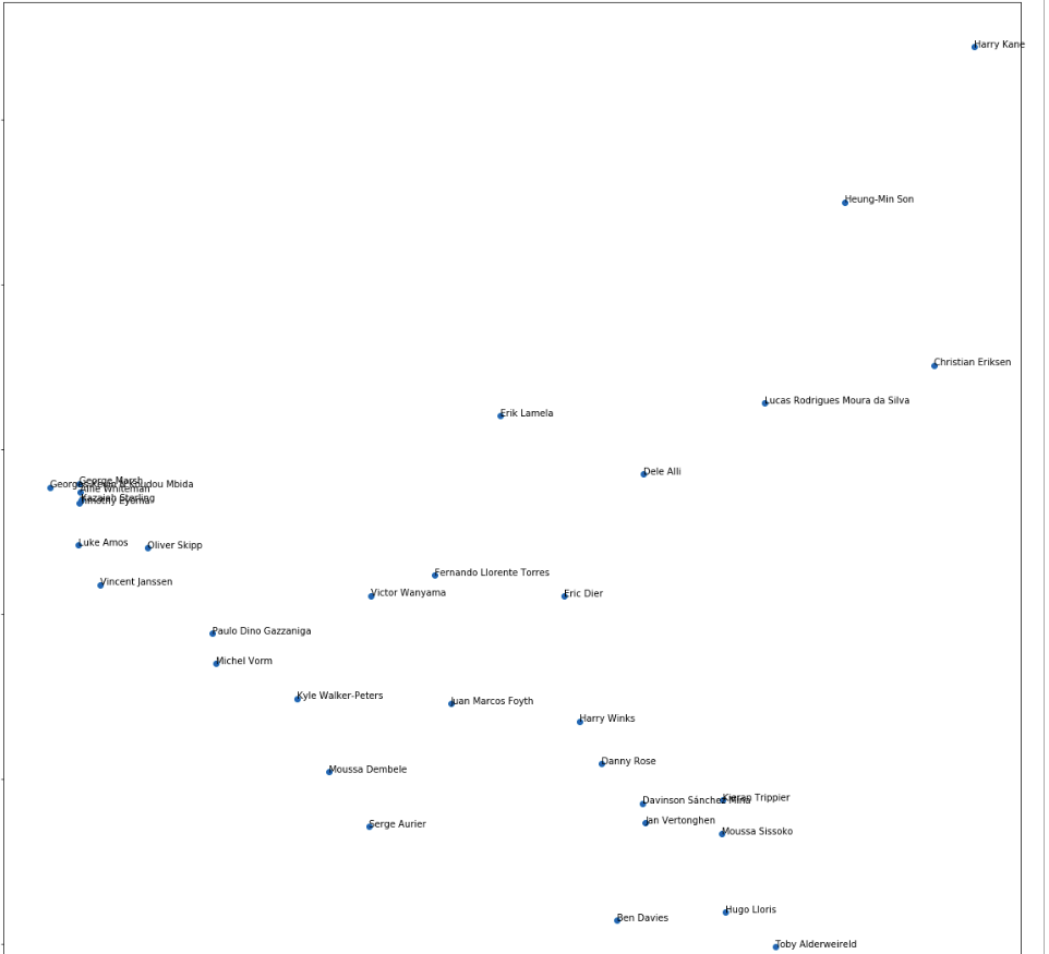
From a quick glance it looks like it’s segregated players based on the playing positions and the duration played across seasons. The players on the far right are largely strikers and attacking players who spent a fair bit of time on the pitch. The center of the graph shows midfielders and holding midfielders with the defenders close to the bottom right and center.

The anomaly is to the far left with the player named Vincent Jannsen who is a striker and didn’t play many games last season. PCA can provide interesting insights on the items during collaborative filtering.